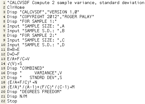
This page will examine and step through multiple solutions
for two sample confidence itnervals
using the TI-83/84 calculators.
Figure 1
|
We are going to create a confidence interval given by
`barx_1 - barx_2 +- t_(alpha/2)*sqrt((s_1^2)/(n_1) + (s_2^2)/(n_2))` using the smaller of
`(n_1-1)` and `(n_2-1)` as the degrees of freedom.
We use this as the "simple method" for determining the number of degrees of freedom.
It is certainly the case that the more complex method, shown later, will give a "higher" degrees of freedom. However, higher degrees
of freedom translate into smaller t-values which in turn yield smaller margins of error which result in
narrower confidence intervals. By using the "simple method" our final result will
be a broader confidence interval, one that will most certainly cover the more compact one found later.
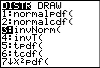
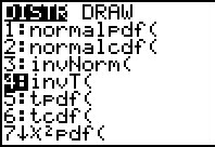
Our first step is to determine the t-value to use for a 99.5% confidence
interval. On a TI-84 (with the newer operating system) we have the invT(
option in the DIST menu (   ). ).
|
Figure 2
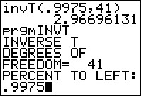 |
The command that we want is invT(.9975,41) where the .9975 comes from
the fact that we want 99.5% inside the confidence interval, leaving
0.5% outside, and that has to be split, half above and have below. Thus,
there will only be 0.25% to the right. The invT( command returns the
t-value having the specified area (for us, .9975) for
all values to the left of the point,
and for the given degrees of freedom. The calculator produces
the t-value: 2.96696131.
For those having a calculator without the invT( option,
we do have the INVT program. This will give approximately the same answer.
In Figure 2 we start the program, giving the required values.
|
Figure 3
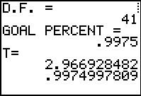 |
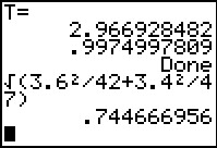
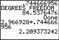
Figure 3 shows the rest of the program output. The value produced is
2.966928428. Not quite as good as the better and faster built-in routine, but
good enough for our purposes. Note that the program also give us the fact that
the value it produced has .9974997809 of the area to its left, not the asked for
.9975.
|
Figure 4
 |
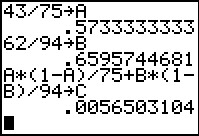
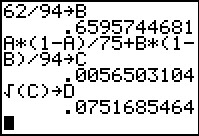
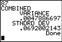
The variance of the difference of the two means
is the sum of the variances of the two means. Since we do not know the
variance of the populations we use the variance of the samples
(which is why we used the t-values rather than use z-scores above).
The desired variance is thus `s_1^2/n_1 + s_2^2/n_2`. This, of course,
makes the standard deviation of the difference of the means be given by
`sqrt(s_1^2/n_1 + s_2^2/n_2)`. For our problem this becomes
`sqrt(3.6^2/42+3.4^2/47`, an expression given in Figure 4. Thus, for this
problem the standard deviation of the sample means is .744666956.
|
Figure 5
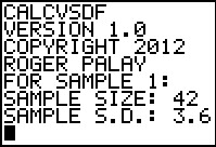 |
Figure 5 shows the start of running the program CALCVSDF,
providing exactly the data from the problem we are doing.
|
Figure 6
 |
Figure 6 completes the data entry.
|
Figure 7
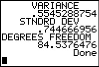 |
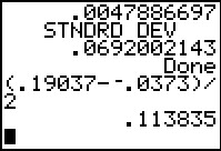
Figure 7 provides the computed results. Note that the display gives both the
variance and the standard deviation,
the latter being exactly what we found back in Figure 4.
|
Figure 8
 |
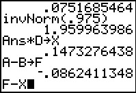
The margin of error is the product of the t-value and
the standard deviation of the difference of the means.
For this problem we actually type in the two values that
we found first in Figure 2 and in Figure 4. [We might note that by reading through the
program we can see that the standard deviation value is stored in the
variable S. Therefore, we could have written the
our expression as 2.966928*S.]
|
Figure 9
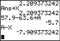 |
In Figure 9 we first store the margin of error in X.
Then we compute the difference in the means,
`x_1-x_2`, and store it in A.
That means that we can get the lower end
of the confidence interval via A-X.
|
Figure 10
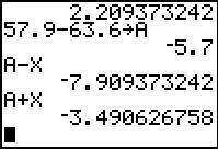 |
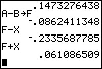
Then, it is easy to get the upper end of the confidence interval from A+X.
Combining these we have the confidence interval as (-7.909, -3.4906).
|
Figure 11
 |
The work done so far has been based, as noted in Figure 1,
on the "simple method" for determining the number of degrees of freedom
that we will use. There is complex formula to derive a larger number of degrees of freedom
which will result in a smaller t=value, thus closing the confidence interval a bit.
This other formula is `(( (s_1^2)/(n_1) + (s_2^2)/(n_2) )^2) / ((((s_1^2)/(n_1))^2)/(n_1-1)+(((s_2^2)/(n_2))^2)/(n_2-1))`.
We would not want to type that into the calculator each time
we solve a problem. However, it is not too much to include it in a program.
That is exactly what was done in the program given above.
Lines 18 and 19 compute the numerator and the denominator of the
expression. Lines 20 and 20 display the result. Thus, back in Figure 7,
we were given the additional information that the
degrees of freedom can be computed to be 84.5376476.
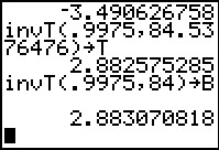
In Figure 11 we have used this strange value with the invT(
command to get a new t-value, namely, 2.883070818,
As expected this is less than the 2.96696131 we found using 41 degrees
of freedom in Figure 2. Note that we not only generate the answer, we
have also stored it in the variable T.
The computed "degrees of freedom" is "strange" in that it is
not a whole number. The TI calculator does not have a problem with this
but we sure are not going to find and and use a table in a text that has
t-values for 2.882575285 degrees of freedom. We take a minute here
to see just how much the t-value changes with slight changes in the degrees of freedom.
For example, if we round down to 84 degrees of freedom we find a value of
2.883070818. This is not much different from 2.883070818.
|
Figure 12
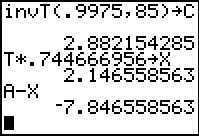 |
In Figure 12 we look at the same computation with 85 degrees of freedom,
generating 2.8821542185, also not much different from 2.883070818.
Then, returning to use the value we stored into the varaible T in Figure 11,
we walk through the same steps that we used in Figures 9 and 10 to find the margin of error,
and store it in X.
This new margin of error is 2.146558563, again smaller than the value we found using
the simple method above.
We go on to find the lower end of the confidence interval.
|
Figure 13
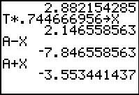 |
And we use A+X to get the upper end.
The new confidence interval, (-7.84656, -3.5534) is indeed narrower
than the interval we found in Figure 10.
|
Figure 14
 |
To this point we have done this problem by following the
formula for finding the confidence interval for the difference of two means.
Now we will do the same problem but we will let the calculator
do all the work.
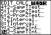
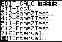
In the STAT menu, under the TESTS submenu, we
find the 2-SampTInt... command. Selecting this command
takes us to the input screen shown in Figure 15.
|
Figure 15
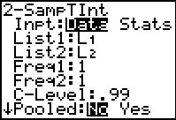 |
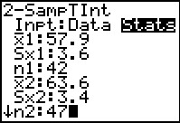
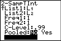
Figure 15 shows the screen as it was found on a particular calculator.
In this case, the input screen is set to input locations of actual Data.
We, however, have a problem that gives us the statistics ,
not the data of the experiment.
We use the  key to move the blinking
highlight over to the Stat option and then
press key to move the blinking
highlight over to the Stat option and then
press to move to Figure 16. to move to Figure 16.
|
Figure 16
 |
Now we have the input screen changed to accept statistic.
We continue by entering the required values:
`barx_1=57.9`, `S_(x_1)=3.6`, `n_1=42`,
`barx_2=63.6`, `S_(x_2)=3.4`, and `n_2=47`.
Then use  to
move down for the remaining settings. to
move down for the remaining settings.
|
Figure 17
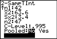 |
Make sure that we specify the given confidence level as
the full 99.5%, entered as .995. Leave the
"Pooled" option on No.
Highlight the calculate option and press .
|
Figure 18
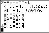 |
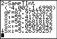
The result, shown in Figure 18, gives the confidence interval (the same as we
found in Figures 12 and 13) and the computed degrees of freedom
that we found (shown in Figure 7 but discussed in Figure 11).
|
Figure 18a
 |
One of the values not shown in the output of the 2-SampTInt command
is the margin of error.
However, since the margin of error is just half the width of the confidence interval
we could calculate it. Such a calculation is shown in Figure 18a.
This should be compared to the 2.146558563 found in Figure 12.
The difference is, of course, due to the use of the rounded
values for the confidence interval in Figure 18.
|
Figure 18b
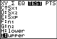 |
We could retrieve the more complete values for the lower
and upper ends of the confidence interval by moving
to the VARS menu, selecting the Statistics option,
and then moving to the bottom of the TEST sub-menu.
To move to Figure 18c we press
to paste the identifier upper onto the main screen.
|
Figure 18c
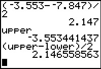 |
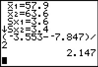
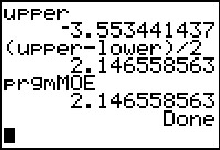
Here we see the longer version of the upper end of the confidence interval
to be -3.553441437.
Figure 18c goes on to form the expression (upper-lower)/2
to generate the same value that we found back in Figure 12.
Typing the expression (upper-lower)/2 takes between 20 and 45 keystrokes,
depending on how you maneuver around the calculator screens. Even at 20 this is an
excessive process. I(f we need to do this many times then this would be a
perfect case for creating a tiny program to just do and display the
computation for us. We will do that.
|
Figure 18d
 |
 gets us to Figure 18d.
From there we use
to move to Figure 18e.
gets us to Figure 18d.
From there we use
to move to Figure 18e.
|
Figure 18e
 |
Here we give the program a name; our name will be MOE.
The calculator starts Figure 18e in alphabetic mode, so press
 
 to generate MOE
Press to move to Figure 18f. to generate MOE
Press to move to Figure 18f.
|
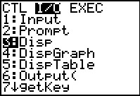
Figure 18f
 |
Here we are ready to write the lines of the program. The only line
we want to construct is Disp (upper-lower)/2.
We use
to move to Figure 18g where we can find the Disp command.
|
Figure 18g
 |
Highlight the Disp command and press .
|
Figure 18h
 |
We have pasted the Disp command into the program.
|
Figure 18i
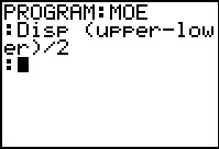 |
Then we go through the 20 to 45 keystrokes to generate the rest of the
command, ending with a .
The program is complete. Press  to get out of the program editor and return to the main screen.
|
Figure 18j
 |
On the main screen we have recalled the program and run it. The output
is what we should expect.
One small warning is appropriate here. The program that we just wrote
uses values that have been stored into upper and lower.
You should use this program immediately after you have
constructed a confidence interval. The program will simply use the values
that it finds in upper and lower. The program will not
recall some much earlier computation of these values.
|
Based upon our samples we want to construct 99.0% confidence intervals for the difference of the two means.
Figure 19
 |
In this case we are given the actual data.
One approach, and the first one used here, is to just
get the statistics that we need and then follow the same path
that we took in the first example.
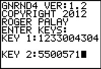
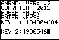
To that end, we generate the data. Note that the generation program, GNRND4,
always generates this data in L1.
Therefore, in order to keep the calculator looking like the problem
that we have been given, we will actually generate the second set of data first.
Then, we will store that data into L2 before
we generate the first set of data.
As a result, when we finally get to Figure 33 we will have the first set of
data in L1 and the second set in
L2.
|
Figure 20
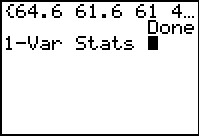 |
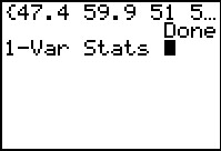
Once the data has been generated, we can do a 1-Var Stats
on it.
|
Figure 21
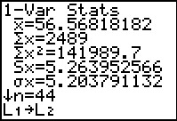 |
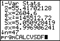
The three values we need are given here, the mean, the standard deviation, and
the sample size. Remember that these are for the second set of data. Therefore we have
`x_2=56.56818182`, `S_(x_2)=5.263952566` and `n_2=44`.
Note that at the bottom of Figure 21 we have copied
L1 to L2.
|
Figure 22
 |
Now generate the first data set. [This will overwrite the data that was in
L1.]
|
Figure 23
 |
Get the statistics for the first data set.
|
Figure 24
 |
Therefore we have
`x_1=55.4170218`, `S_(x_2)=5.050928419` and `n_2=47`.
|
Figure 25
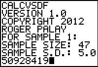 |
Recalling that we can compute the combined variance and standard deviation,
not to mention the complex number of
degrees of freedom, by using the program shown above (between Figures 4 and 5),
we run that program.
Figure 25 shows the start of the program and the first
values that we have entered.
|
Figure 26
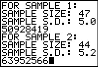 |
Figure 26 shows the rest of the data input for the program.
|
Figure 27
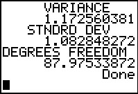 |
Figrue 27 gives us the combined standard deviation, namely, 1.082848272
and the complex number of degrees of freedom, namely, 87.97533872.
|
Figure 28
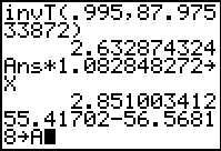 |
Again, following our original path in example 1 above,
we find the required t-value by using invT,
giving it the .995 value (because we split the 1% between the top and the bottom)
and the complex number of degrees of freedom.
That t-value is computed to be 2.632874324.
We then use that answer times the combined standard deviation
to get the margin of error which we store in X as
2.851003412.
Finally, in Figure 28, we compute the difference of the means
and store that in A.
|
Figure 29
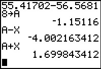 |
Having done all that, we can get the lower and upper ends of the
confidence interval via A-X and A+X, respectively.
|
Figure 30
 |
Alternatively, as we did for the first example, we could just move to the
STAT menu, TEST sub-menu, and choose the 2-SampTInt...
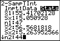
option. This takes us back to our input screen, shown in Figure 30
after we have entered the values for this problem.
|
Figure 31
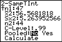 |
Figure 31 shows the rest of the data input,
including setting the confidence level at .99.
Once the values have been entered we highlight the
Calculate option and press .
|
Figure 32
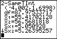 |
The results are given in Figure 32.
At this point we have simply followed the path we laid out in the
first example above. However, the TI calculators
give us another option.
|
Figure 33
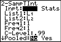 |
We return to the 2-SampTInt screen and change the option back to DATA.
Now the calculator is looking for the raw data.
We tell the calculator that the first list of data is in L1
and the second list is in L2.
These lists contain the data values. There are no associated frequency lists.
Therefore, we leave the Freq1: and Freq2: settings as 1.
Set the confidence level at .99.
|
Figure 34
 |
Move to the Calculate option.
Press to have the calculator do all the work.
|
Figure 35
 |
The results are shown in Figure 35.
|
We are given the following statistics for two independent
random samples of a large population:
Figure 44
 |
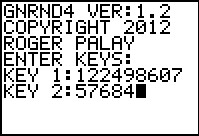
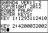
The first thing to do is to generate the data. Here we generate Data Set 3.
|
Figure 45
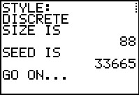 |
Notice that the program reports that it will generate 88 values.
Our particular concern in this problem is the proportion
of 3's in those 88 values. Once the data is generated we need a way to find
the number of 3's in the list.
|
Figure 46
 |
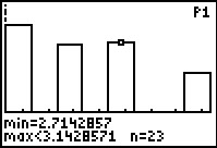
One of the most straight forward methods is to just create
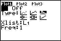
a histogram of the values. In Figure 47 we have moved to the
Plot1 screen and made sure that the plot is ON,
that we will be doing a histogram, and that the data for the
histogram will come from L1.
|
Figure 47
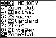 |
We then move to the ZOOM menu and use the
ZoomStat option.
|
Figure 48
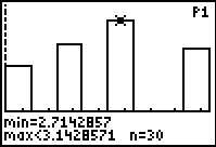 |
Once the histogram is displayed we move to
use the TRACE feature and then move the highlight
onto what we know is the bar for the 3's.
From Figure 48, at the bottom, we see that there are 30
such values in our data.
|
Figure 49
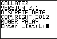 |
An alternative approach is to use the COLLATE2
program. Please note that the version shown here is version 2.1.
This version includes a prompt to let the program complete without displaying all of the
computed statistics.
We tell the program that the data is in L1.
|
Figure 50
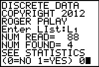 |
The program then tells us that there are 88 items that were found.
This version then asks if we want all of the statistics. Our
response is 0 to indicate "no".
|
Figure 51
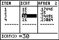 |
After the program has completed we move to the Stat Editor.
Here we find that ITEM 3 has been found 30 times.
Either way approach the problem we now know that the first
list has 30
items that are 3 out of a total of 88 items.
|
Figure 52
 |
Now we can generate the other set of data.
|
Figure 53
 |
Again, we need to find the number of 3's
in this list. Figure 53 uses the histogram method
to do this.
We can see that there are 23 instances of 3
in this data set.
|
Figure 54
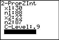 |
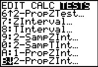
Of course, we could go back through all the steps that we took in Figures
36 through 40 to compute the confidence interval.
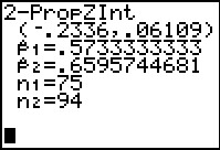
However, using the 2-PropZInt... command will take less time.
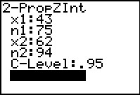
Here we have used that command to open the input form.
Then we go ahead and supply all of the values, including the confidence level.
When all the values are in place we
highlight the Calculate option and press .
|
Figure 55
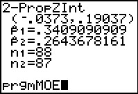 |
The result is the confidence interval given in Figure 55.
Some note should be taken that by using this method we
do not get to see any of the intermediary values such
as the standard deviation
of the proportion difference and the margin of error.
We can take care of the latter by running the program, MOE, that we saw in Figures 18d through 18j.
|
Figure 55a
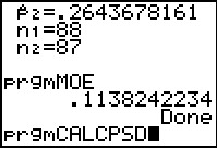 |
This gives us the margin of error based upon the values of lower
and higher that we just computed.
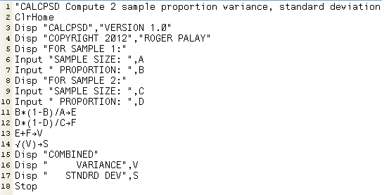
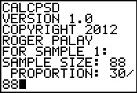
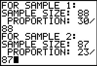
As for the other values, those computations
can easily be placed into a program. Let us look at the listing of the
program CALCPSD given below.
|
We want to construct a 95.0% confidence interval
for the difference between the paired measures.
Figure 60
 |
As usual, we can start by generating the two lists of paired values.
Note that for paired values the GNRND4 program produces lists in
L1 and
L2.
|
Figure 61
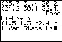 |
The whole idea of the paired values is to derive the difference within each pair.
We do this and store the result in L3.
Then we can look
at the 1-Var Stats
for L3.
|
Figure 62
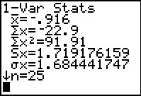 |
This particular problem then resolves to finding the
95% confidence interval for the mean of the difference.
That will be `barx_d +- t_(alpha/2)(s_d)/sqrt(n)`.
We use the values given here to do those computations.
|
Figure 63
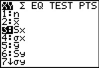 |
To find `s_d/sqrt(n)`, rather than retype the value for `s_d`
we move to the VARS, Statistics menu and select
`S_x`.
|
Figure 64
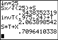 |
Using that we can compute `S_x/sqrt(25)` and store it in S.
Then find the required T-value and store it in T.
Next, find the product S*T, the margin of error, and store it in X.
|
Figure 65
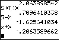 |
We return to the VARS, Statistics menu to retrieve
`barx`. Finally, we form `barx - X` and `barx + X`
to get the limits on the confidence interval.
|
Figure 66
 |
Of course, since this is just getting the confidence interval for the difference of the paired values,
we could have let the calculator do all the work.
We just need to move to the STAT menu, the TESTS sub-menu,
and move down to the TInterval option.
|
Figure 67
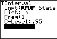 |
This brings up the data input screen. We actually have the data stored in
L3. Making sure that we tell the calculator that the
data is in L3 and that we want a .95
confidence level, we highlight the Calculate option and
press .
|
Figure 68
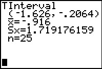 |
The calcualtor does all the work and produces the confidence interval.
|