On this page we will look at a number of examples of one sample hypothesis testing. In particualr, we will look at four different cases outlined in the following table.

Case I: Example 1

Figure 1	We see that the sample mean, `85.284` is indeed greater than the `H_0: mu=77.7`, but is it so big that we will reject `H_0` in a process that will be correct 99% of the time? To find out, we will compute a test statistic, `z=(barx - mu)/(sigma/sqrt(n))=(85.284-77.7)/(13.86/sqrt(26))` and then examine that test statistic. Since we know that the distribution of the sample means is normal, we use invNorm. In this case we look at invNorm(.99) because we want a critical value that represents being too high to be reasonable. Such a value will have 99% or the area under the normal curve to its left. We see that the critical value is 2.326. Then, we compute the test statistic. In Figure 1 we do this in two steps. First we get the eventual denominator and store it in S. Then we compute `(barx-mu)/S` as the test statistic 2.790. Remember that our critical value represented the highest value that we would tolerate and still accept `H_0`. This test statistic is even larger than the critical value. Therefore, we reject `H_0`.
Figure 2	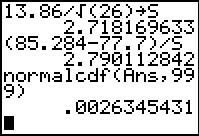The decision that we reached in Figure 1 was based on having the critical value. The P-value approach has us look to see just how much area is to the right of the computed test statistic. We can do this via the normalcdf(Ans,999) command. It returns the value .002634 to indicate that there is less than the 0.01 that we were willing to accept. In the P-value approach, we see that if `H_0` were true, getting a sample with a mean as large as, or larger than, ours would be extremely rare. More rare than the 0.01 we were willing to accept. Therefore, using this method we would reject `H_0`.
Figure 3	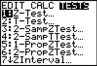We have accomplished a great deal in Figures 1 and 2, but they depend upon our performing many computations. The calculator has a special command that will do almost all of this for us. This is the Z-Test... command found in the STAT menu under the TESTS sub-menu.
Figure 4	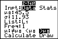The Z-Test... command brings up the data input screen shown in Figure 4. The first thing that we need to change here is that we do not have Data, we have Stats.
Figure 5	Move the highlight to the Stats field and press .
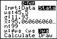
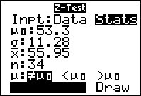
Figure 6	Then move down the form to enter the values: `u_0` is the hypothesized mean, 77.7; `sigma` is the population standard deviation; `barx` is the sample mean; `n` is the sample size; and we want to select `>mu_0` as our test. Then move the highlight to the Calculate option. Press to have the calcualtor perform the test.
Figure 7	Here is the result of that test. The calculator echoes the test, `U>77.7`, produces the test statistic `z=2.790112842`, produces the P-value of that statistic, `p=.00263454431`, echoes the sample mean `barx=85.284` and the sample size `n=26`. It just remains for us to say that the P-value is samller than the allowed 0.01. Therefore, we reject `H_0`.

Case I: Example 2

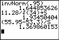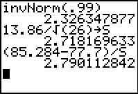
Figure 8	The problem specifies that we will tolerate a 10% error. Therefore, we want critical values that have only 5% below and 5% above them. We use the invNorm(.95) to get those values. Recall that the normal distribution is symmetric. Therefore, our two values are `-1.644` and `1.644`. Our test statistic needs to be outside these values to reject the null hypothesis. Again we compute the test statistic in two steps. The result is 1.369 and this is not outside the critical values. Therefore, we accept `H_0`.
Figure 9	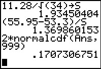Alternatively, we could use normalcdf to find the area to the right of the test statistic. However, we need to remember that we also need to add in the area to the left of the opposite critical value. Again, using the symmetry of the distribution, we compute the total area as 2*normalcdf(Ans,999). The result, 17.07 is larger than the limit that the problem statement imposed. Therefore, we accept `H_0`.
Figure 10	The other approach to this problem is to use the Z-Test... command which opens the input form shown in Figure 10 after we have entered the values from this problem. Highlight the Calculate field and press .
Figure 11	The results, identical to those we found in the longer appraoch, are shown in Figure 11.

Case II: Example 1

Figure 12	The challenge in Case II is that we do not know the standard deviation in the underlying population. In this case we need to use the sample standard deviation whcih changes the distribution of the sample means to a t-distribution, not a normal distribution. Following the process used before, we find the critical value. In this case we may be able to use the invT( command. (This cammand is available on TI-84's with the newer operating system. If it is not available on your calcualtor you may use the INVT program illustratied in Figure 13).
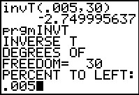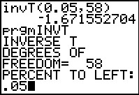
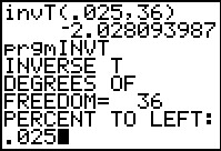
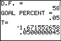
Figure 13	The invT( command, if it is available, has two arguments, the area measure and the number of degrees of freedom. From the problem statement we see that we wnat the area under the curve to be 0.005 and that we have 30 degrees of freedom (one less than the sample size). The result is the value `-2.749995637`. If the invT( command is not available we can use the INVT program. It asks for the number of degrees of freedom and the percent of area to the left. The output from the program appears in Figure 14.
Figure 14	The answer from the program is not wuiote the same as that from the built-in function, but the difference is minor.
Figure 15	Returning to our solution, we compute the test statistic, `t=(barx-mu)/(s_x/sqrt(n))=(13.741-18.6)/(10.02/sqrt(31))`. On the calcualtor we have computed this in two steps, first computing the denominator, then the quotient. The result `-2.69997675` is not as extreme as was our critical value so we accept `H_0`. Alternatively, we could have use the P-value approach where we compute the area outside of the test statistic. We do that with the tcdf( command, wich also requires the degrees of freedom. Again, the result is the 0.0056425488 which is larger than the allowed 0.005 in the problem statement. On that basis we accept `H_0`.
Figure 16	In the TESTS sub-menu of the STAT menu there is a command that does all of this for us, namely, the T-Test... command.
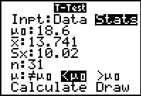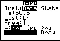
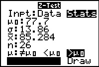
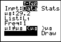
Figure 17	The T-Test... command opens the input form shown in Figure 17. We need to be sure that the Stats option is selected and then we supply the rest of the values as given in the problem, including setting the option for testing the `Calcualte option and press .
Figure 18	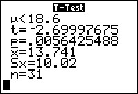Figure 18 gives the results of the command, including the t-statistic and the P-value. The result is the same as we obtained in the longer approach given above.

Case II: Example 2

Figure 19	This second Case II example, the only real change is that we are now looking at a not equal to alternative hypothesis. Therefore, just as we did back in Figure 8, we have to spread the 5% both above and below the supposed mean. Therefore, we find the critical value, using the t-distribution with 36 degrees of freedom, to have 2.5% on each side. Again, in case the invT( command is not available, we can use the INVT program.
Figure 20	We get essentially the same value.
Figure 21	Now we compute the t-statistic as before, producing `-2.600066356`, which is outside of the critical value, resulting in a decision to reject `H_0`. Also, we could have computed the P-value, remembering to double it, to find that it is 0.0134334558 which is far below our threshhold of 0.05.
Figure 22	We could have done the problem using the T-Test... command. We fill in the values from the problem.
Figure 23	The computed results are given in Figure 23.

Case III: Example 1

Figure 24	Case III is similar to Case II, except that we are given the sample, not the sample statistics. This is not much of a problem because we can compute those values. First, we generate the data.
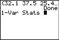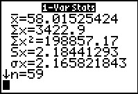
Figure 25	Then, we obtain the 1-Var Stats.
Figure 26	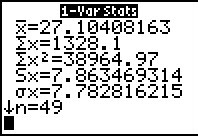The values are given here, and we could write them down and re-enter them later, but we do have an alternative.
Figure 27	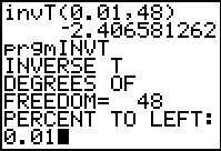As has been our pattern, we first find the critical value either via the invT( command or the INVT program.
Figure 28	Again, the program produces similar results.
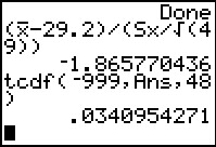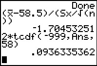
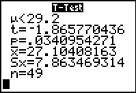
Figure 29	In Figure 29 we compute the t-statistic using the variables from the VARS menu, Statistics... sub-menu. The result, `-1.865770436` is not as extreme as is the critical value. Therefore we accept the null hypothesis. If we compute the P-value we see that it is not strange enough to reject the null hypothesis, which is why we accept it.
Figure 30	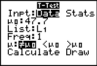The power of the calculator is even more apparent when we use the T-Test... command here. First, we change the setting to Data. This changes the other available options. We just have to tell the command the value to test, the location of the data, and our choice for the kind of test we are running.
Figure 31	Once the values have been set, we highlight the Calculate option and press .
Figure 32	The results are displayed in Figure 32.

Case III: Example 2

Figure 33	For this example we start by generating the data.
Figure 34	Then we compute the sample statistics.
Figure 35	Here is a display of those values. Again, later we will reference the needed values by using the variable names.
Figure 36	Another computation of the critical values, remembering to allocate half the area above and half below, so we use 0.05 instead of the specified 10%.
Figure 37	Here is the alternative method of getting the critical value.
Figure 38	A computation of the t-statistic. The value is more extreme than is the critical value so we will reject the null hypothesis. And a computation of twice the tcdf( also shows that the sample gives a value that is more extreme than we had given 10%.
Figure 39	Use of the T-Test... process requires us to fill in the data form as shown.
Figure 40	The results are given in Figure 40.

Case IV: Example 1

Figure 41	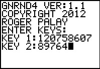Case IV looks at a hypothesis test for a population proportion. We can start by generating the data.
Figure 42	Once the data is generated, and noting that the characteristic of interest is the value 2. All that we really need is to find the number of items and the number of items that are 2. Clearly, one way to do this is to run the COLLATE2 program. We are not really interested in the various statistics that COLLATE2 displays, but we do want to see the table of values along with the count of each item. COLLATE2 is really overkill for this problem. We will look at an alternative method in Figure 51. In order to speed up the process, we have a revision of COLLATE2 program. It is not necessary to use the revised version since it only gives the user a way to skip the slow output of values.
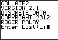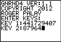
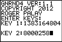
Figure 43	In Figure 43 we can note that we are running version 2.1 of the program.
Figure 44	We note here that there are 87 values. Also, we see the change in the program to allow the user to opt out of the display of values.
Figure 45	After the program completes we move to the Stat Editor. Here we see that item 2 has a frequency of 24. This is all we really need.
Figure 46	As usual, we compute the critical value. Note that we have returned to using the normal distribution. This is because, given the restriction we palce on our sample sizes and the related number of required items in the groups, the distibution of the test statistic will be approximately normal. Another important point, when we compute the denominator of the test statistic we use the proportion from the hypothesis, not the proportion in the sample. [This is different than when we computed the confidence intervals for proportions.] The z-statistic is 1.016492056 which is not as extreme as is the critical value. Therefore, we accept the null hypothesis.
Figure 47	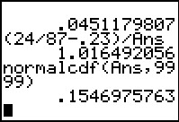In Figure 47 we have computed the area outside of the critical value. It provides a different approach to the problem but produces the same result, we do not reject the null hypothesis.
Figure 48	The TESTS sub-menu of the STAT menu has yet another command, 1-PropZTest..., the command that is appropriate for this case.
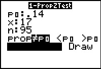
Figure 49	There are few values that we need to supply here. `p_0` is the proportion in the null hypothesis. `x` is the number of items in the sample with the characteristic of interest. `n` is the sample size. And then we have the options for the style of the alternative hypothesis.
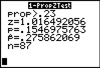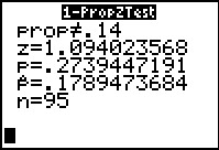
Figure 50	The results are shown in Figure 50. The same values that we computed the long way.
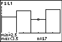
Figure 51	As noted in the discussion along side of Figure 42, once the data is generated, we just need to get a count of the characteristic of interest. In Figure 42 we used COLLATE2 to do this. Here we demonstrate an alternative. We will set up a histogram that will take care of the entire problem. We know that we will have values 1, 2, 3, and 4. We want a histogram that has one column for each value. Set Plot1 be a histogram.
Figure 52	Set the WINDOW valeus to get our separate columns.
Figure 53	Use to move to the Graph. Use to start the Trace. Then use the cursor key to move the highlight to the column of interest, in this case the second column. Note that the number of items in that column is given at teh bottom of the screen. We will use this approach for the next example.

Case IV: Example 2

Figure 54	Generate the data.
Figure 55	Find the critcal values, remembering to split the area onto both the left and right.
Figure 56	Because the Plot1 and WINDOW values have been set, use to open the graph. Then, using the TRACe faciltiy, we find that the value of interest has 17 values. [Somewhere in here we needed to figure out that the sample size was 95.]
Figure 57	Compute the required denominator using the value from `H_0: p=.14`. Get the z-statistic. Compare it to the critical value. The z-statistic is not as extreme as is the critical value. Therefore, we accept the null hypothesis. When we compute the area under the curve that is more extreme than the z-statistic, we see that there is too much area out there to reject the null hypothesis.
Figure 58	Alternatively, we could use the 1-PropZTest to do all of the work, but we need to know the number of items that have the characteristic of interest and the sample size.
Figure 59	And we have the results.