Group Data
This page is devoted to presenting, in a
step by step fashion, the keystrokes and the
screen images for getting 1-Var Stats based on
Group data on a TI-83 (TI-83 Plus, or TI-84 Plus) calculator.
After presenting the problem, we will do the analysis at multiple times
and even in different ways.
To demonstrate these steps we need to start with some data.
We are given the following table of sample data:
| Table 1 |
Class
Lower
Limit |
Class
Upper
Limit |
Number
in
Class |
| 274 | 284 | 5 |
| 284 | 294 | 7 |
| 294 | 304 | 18 |
| 304 | 314 | 9 |
| 314 | 324 | 9 |
| 324 | 334 | 7 |
| 334 | 344 | 11 |
| 344 | 354 | 11 |
| 354 | 364 | 2 |
We can see, from that data, that there were 79 original data points.
However, we have only been given the grouped data. Nonetheless,
we can use that data to get approximations of the sample statistics
of the original data. To do this, we want to choose the
midpoint of each class as the representative value of that class.
Once we have done that then we process the data in the same way that we had
earlier processed One Variable Grouped Discrete data.
Our first step is to get the midpoint of each class in Table 1.
Fortunately for us, the class width given to us is a nice even value, namely 10,
and the class lower limits are also nice integer values. It should not be
too much for us to modify the original data to produce the following:
| Table 2 |
Class
Lower
Limit |
Class
Upper
Limit |
Class
Midpoint |
Number
in
Class |
| 274 | 284 | 279 | 5 |
| 284 | 294 | 289 | 7 |
| 294 | 304 | 299 | 18 |
| 304 | 314 | 309 | 9 |
| 314 | 324 | 319 | 9 |
| 324 | 334 | 329 | 7 |
| 334 | 344 | 339 | 11 |
| 344 | 354 | 349 | 11 |
| 354 | 364 | 359 | 2 |
If we were to follow the directions in the textbook, our next steps would be to
add a row to the table to hold,
at the bottom of the Number in Class column,
the sum of the frequencies, that is, to hold the value 79.
Then we would add a column to hold the product of the frequencies and the
class midpoint values.
Would use the last row of that column to hold the total
of the frequencies times the class midpoints.
Then, from that information we could
compute the mean of the data (the sum from this last column divided by the sum of the Freq column).
For the numbers in our table that would be 25041/79=316.9746835.
We would use that mean value as an approximation to the mean of the data that
first generated Table 1.
The table now appears as
| Table 3 |
Class
Lower
Limit |
Class
Upper
Limit |
Class
Midpoint |
Number
in
Class:
Freq |
Freq*Midpoint |
| 274 | 284 | 279 | 5 | 1395 |
| 284 | 294 | 289 | 7 | 2023 |
| 294 | 304 | 299 | 18 | 5382 |
| 304 | 314 | 309 | 9 | 2781 |
| 314 | 324 | 319 | 9 | 2871 |
| 324 | 334 | 329 | 7 | 2023 |
| 334 | 344 | 339 | 11 | 3729 |
| 344 | 354 | 349 | 11 | 3839 |
| 354 | 364 | 359 | 2 | 718 |
| | | | total: 79 | total: 25041 |
Thereafter, we add another column to hold the difference between
the midpoint and the calculated mean.
Then we add a another column to hold the square of
the calculalted difference between the midpoint and the calculated mean.
Finally, we add a column that is the frequency times the square of the differences
between the midpint and the calculated mean.
We get the sum of the values in this last column.
The table now appears as
| Table 4 |
Class
Lower
Limit |
Class
Upper
Limit |
Class
Midpoint |
Number
in
Class:
Freq |
Freq*Midpoint |
Midpoint
–
Mean |
Square
of
Mid - mean |
Freq *
(Mid - mean)² |
| 274 | 284 | 279 | 5 | 1395 | -37.97 | 1442.1 | 7210.4 |
| 284 | 294 | 289 | 7 | 2023 | -27.97 | 782.58 | 5478.1 |
| 294 | 304 | 299 | 18 | 5382 | -17.97 | 323.09 | 5815.6 |
| 304 | 314 | 309 | 9 | 2781 | -7.97 | 63.596 | 572.36 |
| 314 | 324 | 319 | 9 | 2871 | 2.025 | 4.102 | 36.917 |
| 324 | 334 | 329 | 7 | 2023 | 12.025 | 144.11 | 1012.3 |
| 334 | 344 | 339 | 11 | 3729 | 22.025 | 485.11 | 5336.3 |
| 344 | 354 | 349 | 11 | 3839 | 32.025 | 1025.6 | 11282 |
| 354 | 364 | 359 | 2 | 718 | 42.025 | 1766.1 | 3532.3 |
| | | | total: 79 | total: 25041 | | | 40275.9 |
The quotient, 40275.9/(79-1)=516.35, is the variance of the grouped data, assuming this is a set of sample data.
The square root of that is 22.7235, which is then the standard deviation
of the grouped data. We would use that value as an approximation to the
standard deviation of the original data that generated table 1.
That is a great deal of work. The calculator can do this for us in just a few steps.
First, we need to get the required values into the calculator. Those required values are just the
class midpoint values and the class frequencies. We can store those two
lists in L1 and L2.
Figure 1

|
We will start the process by making sure that we have a "clean" and "set up"
calcuulator. We open the Memory menu via the
  keys.
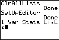
From here we will select the fourth option, ClrAllLists,
by pressing the keys.
From here we will select the fourth option, ClrAllLists,
by pressing the  . This will paste that
command onto our main screen. . This will paste that
command onto our main screen.
|
Figure 2
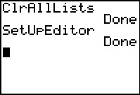 |
Once the command is pasted here we press  to have the calculator perform the command. This has made sure tht there is no
data in any lists that are on the calculator.
to have the calculator perform the command. This has made sure tht there is no
data in any lists that are on the calculator.
Our next step is to
make sure tht we set up the stat editor.
To do this we press  to open the
STAT menu, then press to open the
STAT menu, then press  to select and paste teh SetUpEditor command, and finally, on the main
screen, press to perform the command.
This has made sure that the StatEditor si
set to display the six built-in lists, starting with L1.
to select and paste teh SetUpEditor command, and finally, on the main
screen, press to perform the command.
This has made sure that the StatEditor si
set to display the six built-in lists, starting with L1.
|
Figure 3
 |
In fact, our next step will be to move to use the StatEditor
so that we can put the list of midpoint values into L1.
Press to open the STAT menu, then press
to start the Edit... process. Figure 3
shows the editor set up just as we have arranged.
We proceed by entering the nine numbers for the midpoint values
(279, 289, 299, 309, 319, 329, 339, 349, and 359).
|
Figure 4
 |
We have captured Figure 4 just before we press
to accept 329 as the sixth value. The first five are shown on the screen.
|
Figure 5
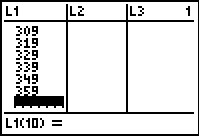 |
Figure 5 shows the screen after all 9 values have been entered. Note that the calculator is
in position to enter a tenth. We do not have a tenth value to enter. Instead we want to
start entering the frequencies into L2.
Therefore, we press the  to move to the next column. to move to the next column.
|
Figure 6
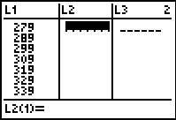 |
Now, positioned in the L2 column,
we can enter the frequencies (5, 7, 18, 9, 9, 7, 11, 11, and 2).
|
Figure 7
 |
Figure 7 shows the list after we have entered six values and as we are
about to enter the seventh.
|
Figure 8
 |
All of the values have been entered. We can safely exit the editor via the
 sequence. sequence.
|
Figure 9
 |
The command that we want to use is 1-Var Stats L1,L2.
That command will instruct the calculator to perform the 1-Var Stats
using the values found in L1 along with the
associated frequencies found in L2.
We start constructing that command by going to the STAT menu via
, then using
to move to the CALC sub-menu, shown in Figure 9, and then pressing
 to select the desiored command and have it pasted onto the main screen. to select the desiored command and have it pasted onto the main screen.
|
Figure 10
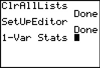 |
Now that the start of the command is here we contnue constructing the command
with L1
 L2.
L2.
|
Figure 11
 |
Note how the calculator wraps the command onto a second line. If we were using
a TI-84 Plus with MathPrint turned ON then this wrapping of commands would be
replaced by a scrolling left and right feature.
Once the command is created we press
to have the calculator perform it.
|
Figure 12
 |
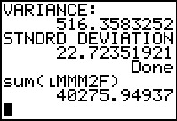
Here we have all the answers, and more, that we worked so hard to get in
the various tables at the start of this problem. The mean is
given as 316.974835, and, since this is sample data, the
standard deviation is 22.72351921. The calculator even gives us the sum of all the values
as 25041. It is interesting to note that the calculator does not
provide us with the other total we used above, namely,
40275.9. This is because there is another, equivalent, formula for
finding the standard deviation, and it uses the sum of the squares of the
values which is displayed here as 7977639.
|
Figure 13
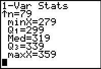 |
We can also use the  key to see the rest of the descriptive values. key to see the rest of the descriptive values.
|
The calculator method requires little of us. From the original problem statement
in Table 1 we had to
- find the midpoint values (Table 1 only had the Low
and HIGH values)
- enter the midpoint values into the calculator
- enter the frequency values into the calculator
- create and run the 1-Var Stats
L1,L2 command
Of these tasks, finding the midpoint values and then entering the values was the most
tedious part. Perhaps we can automate that. To get the
midpoint values we need to know the lower limit of the first class
and the class width. Knowing that and the number of classes that we want,
all we need to do is to find add half the class width to the lower limit to get our
first midpoint and then add the class width to that value
over and over to get the subsequent midpoints. The program GRPAPPX
does this and more. Once it has those values the program asks for the individual
frequency values. Once they have been entered the program does the calculations
needed to obtain the desired statistics and it displays those values. Let us
do the problem again, this time using GRPAPPX.
Figure 14
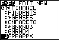 |
We move to the list of programs via the
 key, and then we move down,
using the key, to find the desired program.
On the calculator used here the program was so far down the list that
the only way to select it is to move the highlight to that program,
as shown in Figure 14, and then press the
key. key, and then we move down,
using the key, to find the desired program.
On the calculator used here the program was so far down the list that
the only way to select it is to move the highlight to that program,
as shown in Figure 14, and then press the
key.
|
Figure 15
 |
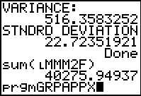
This pastes the command prgmGRPAPPX onto the screen.
We press to actually start running the program.
|
Figure 16
 |
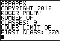
The program first asks for the number of classes.
We had Table 1 as our starting point in the problem, so we know that there are
9 classes. Therefore, we respond with 9.
Then the program asks for the lower limit of the first class. Again,
from Table 1 we know this is 274.
|
Figure 17
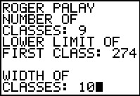 |
The program moves on to ask for the class width. We can see that the width is 10 and we enter that value.
(It is worth noting that we could have let the calculator determine this
value by entering 284–274.)
|
Figure 18
 |
The calculator then prompts us for the frequencies in each class.
Figure 18 shows this after we have entered the frequencies of the first five
classes and before we enter the frequency of the sixth class.
Two important point should be made here. First, in an attempt to
make the program pretty, the programmer got GRPAPPX to construct each of
the prompts with text and class number. This takes time.
Therefore, the program is not as fast as is the usual user.
It is easy to get ahead of the program, trying to enter a frequency value
here before the calculator has asked for it. In that case, the calcualtor will not
record the key you have pressed and you will have an incorrect entry.
Second, unlike the editor, you cannot go back to correct an entry in this program.
Once a value is entered and you have moved to the next value, you cannot change
what has been entered. If that happens, all you can do is to stop the program and start all over again.
|
Figure 19
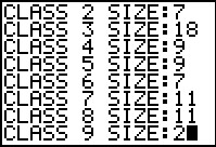 |
Figure 19 shows the program as we are about to enter the final frequency.
|
Figure 20
 |
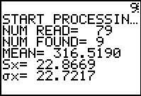
The program accepts tht last frequency value, does all of the calculations,
and starts to produce the output.
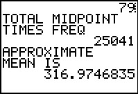
The 79 at the top of the screen was the number of items found.
The 25041 is supplied for reference.
The mean of the data, in this case 316.9746835, is given. It is the exact mean of the
data we have, but it is noted as an approximation because we are
using this as an approximation to the mean of the
data that originally created Table 1.
The program is in a paused condition, press
to continue.
|
Figure 21
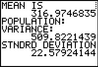 |
In case this represents a population the program
displays the variance and the standard deviation values.
THis is probably overkill since there is little reason to
believe that we should ever consider this to be a population.
After all, the values in Table 1 are not the original 79 values.
We are not using the original 79 values, we are using the midpoint of the classes
to do our computations. Nonetheless, the
program can do the calculations and present the results. It is up to
the user to
know which resutls to use. It is more likely that we should use the
sample statistics. To get those we press
to allow the program to continue.
|
Figure 22
 |
Here we have the variance and standard deviation treating the data as
coming from a sample.
The standard deviation shown here is the same value
that we found above, in Figure 12.
However, in this case, the program also tells us the variance.
Usually we do not worry about how a program actually computes the valeus that it does.
We are satisfied if the program just produces the right results.
We do know that the results of Figrue 12 came from the
calculator's 1-Var Stats command. THe results shown in Figures 21 and 22
came from the GRPAPPX program, and the results match the earleir results.
Still, it will be slightly instructive to see the methodology of the
GRPAPPX program.
|
Figure 23
 |
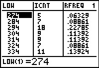
We return to the StatEditor
via . Here we see that the first three
columns are given the names
- LOW to hold the lower limit of each class
- MDPT to hold the midpoint of each class
- FREQ to hold the frequency for each class.
The valeus in the lists are appropriate for our problem.
|
Figure 24
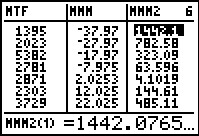 |
Using to move to the right so that we can see the
next three lists we find
- MTF to hold the midpoint times the frequency
- MMM to hold the midpoint minus the mean
- MMM2 to hold the square of the midpiont minus the mean.
|
Figure 25
 |
Again, moving to the right we see the final column
- MMM2F to hold the frequency times the square of the midpoint minus the mean
These are the columns that we used in Table 4.
It was from these values that we found the sum of the final column
and from that sum we found the variance. Now, rather than have us actually add the values in that final
column, we can get the calculator to do taht for us.
|
Figure 26
 |
We left Figure 25 via the
sequence. We then move to the LIST menu via the
key sequence,
and from there, using ,
we move to the MATH sub-menu, shown in Figure 26.
We want the fifth option, sum(. To get that we presss the
key.
|
Figure 27
 |
That pastes the start of the command onto the screen.
We want the calculator to find the sum of the valeus in MMM2F. We need to find that name.
|
Figure 28
 |
Return to the LIST menu. Move down the list of names until we find MMM2F.
Then we can select the highlighted name by pressing the key.
|
Figure 29
 |
Complete the command by adding the closing parenthesis via the  key.
(Note that the actual name pasted by the calcualtor is slightly different from the item we selected.
That difference is the leading small L. This is the character
that the calculator uses to denote a list name at various times.)
We can press to hav ethe calculator perform the command. key.
(Note that the actual name pasted by the calcualtor is slightly different from the item we selected.
That difference is the leading small L. This is the character
that the calculator uses to denote a list name at various times.)
We can press to hav ethe calculator perform the command.
|
Figure 30
 |
The result, shown in Figure 30, is the same value that we got back in
Table 4. From that we could calculate the sample variance by dividing that value
by (79-1), that is, by 78. We could get the standard deviation
by taking the square root of that answer.
|
A quick review of our progress thus far reveals that
before we even started the problem there was some set of 79 values.
We have not seen those values. We start the problem with a frequency table that
has equal width classes aand that gives us the lower limit of each class and the frequency of each class.
From this we can determine approximate values for the mean,
variance, and standard deviation statistics of the original 79 values.
Having done this work, we are just about ready to turn in our results when the
person who gave us the original table returns to tell us that, on second thought,
it would be better if the classes had "nicer" boundaries. Therefore, we now have a new table
and we need to redo our work. The new table is
| Table 5 |
Class
Lower
Limit |
Number
in
Class |
| 270 | 1 |
| 281 | 10 |
| 292 | 18 |
| 303 | 10 |
| 314 | 9 |
| 325 | 10 |
| 336 | 11 |
| 347 | 8 |
| 358 | 2 |
We smile and go back to work, wondering if this is going to change our answers.
Figure 31
 |
We might as well use the program. Return to the list of programs and again
select GRPAPPX. This pastes the name onto the main screen.
Use to start the program.
|
Figure 32
 |
Enter the number of classes, 9, and the first class lower limit, 270.
|
Figure 33
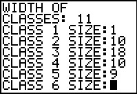 |
Then enter the width of the classes, 11,
followed by the frequency for each class.
|
Figure 34
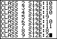 |
Finish entering the frequencies.
|
Figure 35
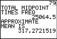 |
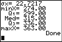
The new approximate mean is 317.2721519. This is different from the mean that we
got from Table 3 (although it was presented just above the display of that table),
Figure 12, and Figure 20. This approximate mean is based on a different organization of the original data.
Both answers are good. Both are good approximations.
Had we been given the original 79 values then we could have actully
found their mean.
This is the best we can do with the data that we have.
|
Figure 36
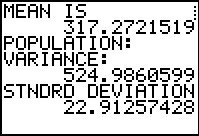 |
We continue to find the population variance and standard deviation.
|
Figure 37
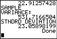 |
And then to find the sample variance and standard deviation. These are new values. They are
close to but not identical to the values that we found before.
They remain good approximations to the true value.
|
Since it did not take much time to get our approximtions,
we decide to provide a historgram of the data in Table 5.
Figure 38
 |
In preparation for this we will return to the StatEditor
just to verify the values there. We use the keys
to get to Figure 38.
We will be happy if we can get a histogram using the values in MDPT and
FREQ. We could safely exit Figure 38 via
.
|
Figure 39
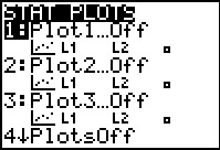 |
Use  to open the STAT PLOT menu.
This particualr claculator has all of the plots turned Off.
Plot1 is highlighted. Pressing will open
the settings for Plot1. to open the STAT PLOT menu.
This particualr claculator has all of the plots turned Off.
Plot1 is highlighted. Pressing will open
the settings for Plot1.
|
Figure 40
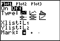 |
Figure 40 shows the initial settings for Plot1 on this calculator.
We want to change these to On, the Type:
needs to be  ,
Xlist: needs to be our MDPT list, and
Freq: needs to be our FREQ list. ,
Xlist: needs to be our MDPT list, and
Freq: needs to be our FREQ list.
|
Figure 41
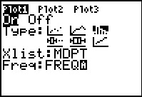 |
For Figure 41 we have made these changes. Before we leave this Figure, note that
we just typed the names of the two lists for this. That is, the calculator had
already put itself into alpha mode (note the  blinking cursor). It was sufficient to press
 
  to generate the FREQ.
An alternative approach would have been to go to the
LIST menu and to find and select the names that we needed here.
Had we done tht then the names here would have had the initial
L in front of them. to generate the FREQ.
An alternative approach would have been to go to the
LIST menu and to find and select the names that we needed here.
Had we done tht then the names here would have had the initial
L in front of them.
However we achieve the changes, once the settings
have been changed we do a ZoomStat, via  . This will take us to the graph in Figure 42.
|
Figure 42
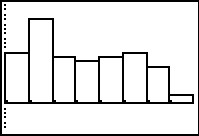 |
This is the histogram that the ZoomStat command determined by
computing new values for the
WINDOW settings. This is an accurate histogram, but not the one we want.
For one thing, this hs only 8 columns and we want a different column
for each of our 9 classes. For another, we know that the list of frequencies
is 1, 10, 18, 10, 9, 10, 11, 8, and 2. That is a bit different that the image here.
|
Figure 43
 |
If we move into TRACE mode, via  ,
the calculator telss us the limits on the first "classs", as well as the fact that the first class has
11 values in it. We see, from the limits on the first class of 275.5 to 288.07143
that the first class deterined here contains both of our first two classes, one with a midpoint of 275.5
and the other with a midpoint of 286.5. We can solve this issue by returning to the WINDOW
settings and putting in our own values. ,
the calculator telss us the limits on the first "classs", as well as the fact that the first class has
11 values in it. We see, from the limits on the first class of 275.5 to 288.07143
that the first class deterined here contains both of our first two classes, one with a midpoint of 275.5
and the other with a midpoint of 286.5. We can solve this issue by returning to the WINDOW
settings and putting in our own values.
|
Figure 44
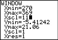 |
We get to the WINDOW settings via the  key.
In Figure 44 we ahve already changed the Xmin to 270, the
Xmax to 369, and a new Xscl set to 11. With these values in
place we can return directly to the graph via key.
In Figure 44 we ahve already changed the Xmin to 270, the
Xmax to 369, and a new Xscl set to 11. With these values in
place we can return directly to the graph via  . .
|
Figure 45
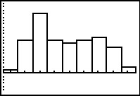 |
Here is the revised histogrm and it looks just the way we would expect.
|
Figure 46
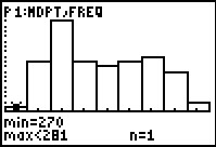 |
Returning to TRACE mode, via ,
we see the limits of the first class and the fact that there is just 1 value in that class.
|
Figure 47
 |
Moving to the right via we see the limits of the second
class and the fact that there are 10 items in that class.
We could continue to scan across the columns to see the values in each
class.
|
As it turns out, the backgound data, the 79 values, that went into the
making of both Table 1 and Table 5 came from a run
of the GNRND4 program. It will be instructive for us to look at the real
set of values and to determine the actual mean and standard deviation of those values.
That way we can compare the approximations that we found above to the real
statistics (parameters) of the original sample (population).
Here is a table of the original vlaues:
Figure 48
 |
We start by running the GNRND4
program and giving it the necessary key values.
|
Figure 49
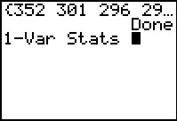 |
The program completes. The values are now
stored in L1.
We get the 1-Var Stats command.
Left alone this will do the analysis of the data in L1.
That is what we want. Press to start the actual processing.
|
Figure 50
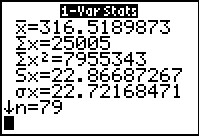 |
The result gives us the true mean, 316.5189873, and the
standard deviation if this is a sample of some data, 22.86687267, and the
standard deviation if this is a population, 22.72168471.
We can see that our earlier approximations were really quite good.
|
Figure 51
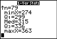 |
We move down to see the rest of the information from
1-Var Stats.
|
Figure 52
 |
Just to confirm that the data of Table 6
would be grouped as in Table 1, we run the COLLATE3
program giving it L1 as the source for the data.
|
Figure 53
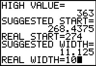 |
We set the lower limit of the first class to be 274
and we set the class width as 10.
|
Figure 54
 |
The program displays the values shown. Remember that these values have been rounded
to 4 decimal places.
|
Figure 55
 |
The program concludes. In order to really seen the values that we need to
confirm Table 1 we will go tot he StatEditor.
|
Figure 56
 |
In Figure 56 we see exactly the same lower limits
and frequencies that we had in Figure 1, at least through the
first 7 rows of the table.
|
Figure 57
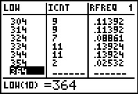 |
We conclude by moving down the editor screen to see and verify the last two rows of
the table.
|
©Roger M. Palay
Saline, MI 48176
September, 2012