This page is devoted to presenting, in a step by step fashion, the keystrokes and the screen images for examining a Discrete Distribution on a TI-83 (TI-83 Plus, or TI-84 Plus) calculator. This will include entering the information, processing it by brute strength and awkwardness to get the expected value (the mean), and the variance and standard deviation. Then we will do the same computations using the built-in function of the calculator. In the process we will look at a small bit of the math behind some of this.

To start we are given the probability distribution for a discrete variable. The following table does this:

Figure 1	In earlier pages we have used the StatEditor to enter data into the calculator. In this demonstration we will enter the values directly into the two lists, L1 and L2. It is a good idea to set up the editor and to clear all prior data from the lists on the calculator. The sequence will select, paste, and perform the SetUpEditor command. The sequence will select, paste, and perform the ClrAllLists command. To store the list of data values from the table above in L1 we enter the values, enclosed in curly-braces and separated by commas and then store that into the desired list. The key seequences is . The display should appear as in Figure 1.
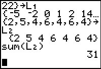
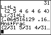
Figure 2	Having entered the command we press to have the calculator perform it. The calculator not only stores the values, it also displays the list on our screen, this time without the commas. Our next task is to enter the probabilities into L2. Again we will enter these directly. However, since all of the values have a denominator of 31 we will just enter the numerator at this time. Therefore, the lsit that we want to assign to L2 is {2,5,4,6,4,6,4}. We press the keys to generate that list and then use the key to assign it to L2. The calculator redisplays the values.
Figure 3	Naturally we want to be sure that we have entered the right values. We can do this by inspection, looking at the values both in the original table and on the calculator screen. In this case we can do a bit more than that. We know that the probabilities have to add to 1. We also know that we still have to divide each of the values in L2 by 31. Therefore, we if we entered the values correctly into L2 then the sum of those values needs to be 31. We can instruct the calculator to find the sum of the values in a list. We move to the LIST menu via . 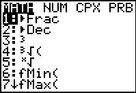Then we move to the MATH sub-menu. The command that we want is the fifth one, sum(. We press to select that command and paste it onto the main screen.
Figure 4	Then we complete the command with and have it performed via . We are happy to see that the sum is indeed 31.
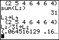
Figure 5	In preparation for a discussion below we will make a copy of L2 in L4 by using . Then we can take care of dividing each value in L2 by 31 by using . The calculator again displays the result, but given the values involved the individual numbers use so many digits that we really only see one probability value at a time. We could ask the calculator to display the values in fractional form.
Figure 5a	We open the MATH menu via . We want the option. Therefore, press .
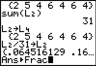
Figure 5b	The result is that the calculator supplies the ANS, representing the previous answer, and then appends the option. Press to perform the task.
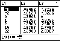
Figure 5c	We now see the values that have also been stored in L2 in fractional form. Another way to look at the values is to use the StatEditor.
Figure 6	We open the StatEditor with . Here we see both the data values of L1 and the probability values, to 5 decimal places, in L2.
Figure 6a	Using brute strength and awkwardness, we can find the expected value which is also the mean value, by multiplying each value in L1 by its matching probability in L2, and then adding all of the answers. The command shown in Figure 6a, built via , accomplishes the first part of this, multiplying the specific values and putting the separate products into corresponding elements of L3.
Figure 7	To get the sum of all the values in L3 we return to the LIST menu and move to the Math sub-menu to find sum( as option number 5. Press to paste that command to the main screen.
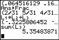
Figure 8	complete the command with . The calculator does the task and gives the answer as 5.35483871.
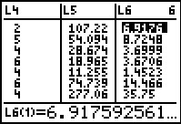
Figure 9	We want to save that result in the variable X, just in case we might want to use it later. To do this we can press . The calculator supplies the Ans seen on the screen. Press to perform the command. To get the variance of the data we want to start by finding the squared differences between the data values and the mean. The command (L1–X)2 will do this. We create that command and store the resutls in L5 via . Then press to perform the command. The calculator displays the results after it stores them in L5. 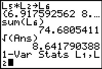Then we want to multiply those values by the probability values stored in L2. The key sequence creates and performs the command, putting the results in L6.
Figure 10	Now that we have the individual values we need to find the sum of all of them. We return to the LIST menu via , move to the MATH sub-menu via , and then select the fifth option, sum( via , and finish the command with and then with . With that we find that the variance is 74.6805411. To get the standard deviation we just need to take the square root of the variance. Press and then, to recall the answer we just calculated, and finish with . From this we see that the standard deviation is 8.641790388.
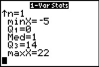
Figure 11	So much for the brute strength and awkwardness approach. It was nice to see that we could follow the definitions of the mean, variance, and standard deviation to get results. However, the calculator will really do this for us. In Figure 11 we have moved to the STAT menu and then the CALC sub-menu via . We select and paste the 1-Var Stats command by pressing .
Figure 12	We need to complete the command to read 1-Var Stats L1,L2. It is essential that we augment the command with the names of the two lists, the first holding the vlaues of the original table and the second holdign the probabilities for those distinct values. Then we press to have the calcualtor perform the command.
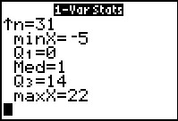
Figure 13	The results, shown in Figure 13, verify the values of the mean and standard deviation that we found above. There are two features of this display that need to be addressed. The first is that the indicated value of n is 1. The computation of the value of n is to add all of the values in the second list in the command, in this case, add all of the values in L2. Of course, those are all probabilities and we know that the sum of the probabilities asssigned to all the distinct values has to be 1. The second feature is that there is no value given for Sx. This will happen when the two lists that we give to the 1-Var Stats command represent discete values and their associated probabilities. (Actually, it seems that the calculator refrains from giving the values of Sx if the value of n is not a whole number greater than 1. This makes some sense because that is a clear indication that the values of the frequencies are not really frequencies.)
Figure 14	Somewhat in preparation for a further discussion, we have moved down the screen, using to see the rest of the output from the 1-Var Stats stats command.
Figure 15	Recall that in Figure 5 we made L4 hold a copy of the original values that we put into L2, namely, the numerators of all the probabilities given in the original table. We will return to this now. We reconstruct the 1-Var Stats command but this time we use 1-Var Stats and L4. Then we have the calcualtor perform the command.
Figure 16	The results are amazingly similar to those of Figure 13. In particular, the value of `barx=5.35483871` and the value of `sigma_x=8.641790388`. The other values have certainly changed, including the value `n=31`. Before we examine this in detail, let us look at some more of the output.
Figure 17	Here we have moved down the display to see the rest of the output from 1-Var Stats. These last five values are identical to those that we saw in Figure 14.
Figure 18	Figures 18 and 19 are provided just to confirm the contents of all of the lists that we have used.
Figure 19	Figures 18 and 19 are provided just to confirm the contents of all of the lists that we have used.

At this point in the coruse we have used the terms mean, variance, and standard deviation in two seemingly different settings. Earlier we looked at those values for a set of data points and we had a formula for calculating each of them. Now we are looking at discrete data points and respective probabilities. We have a formula for the three values, mean, variance, and standard deviation, in this setting. The challenge for many students is that the formuli look different. The following table presents the formuli as they have been given.

We will go through a lengthy explanation of the equivalence of the two formuli for the mean. This explanation then becomes the model for understanding the equivalence of the other formuli.

We have the formula for `n` data points as `mu = (Sigma_(i=1)^n(x_i))/n`. If we construct a frequency table for those data points we find that we have `m` distinct values and a frequency associated with each of them. We will name that frequency `F(x_k)` where `k=1,2,3,...,(m-1),m`. Consider the following data set

Alternatively, we could create a frequency table for the same data:

Using the same approach, for the variance we have `sigma^2 = (Sigma_(i=1)^n(x_i-mu)^2)/n` for `n` data points. However, if we have a frequency table for `m` distinct values in those `n` data points, and we have the frequencies represented by `F(x_k)` then we could rewrite that as `sigma^2 = (Sigma_(k=1)^m(x_k-mu)^2*F(x_k))/n`. That can be rewriten as `sigma^2 = Sigma_(k=1)^m((x_k-mu)^2*(F(x_k))/n)`. Again, we can replace `(F(x_k))/n` by `P(x_k)` and we get `mu = Sigma_(k=1)^m(x_k*P(x_k)) - mu^2`.

The equivalence for the standard deviation formuli follows the same way. We just have everything under the square root sign.