This page is devoted to presenting an example of doing a hypothesis test and, in that process, presenting the use of the ASTUDT program as a replacement for the INVT program and as a calculator replacement for using a table of values.
The problem that we will examine here is to test, for a given population, the null hypothesis:
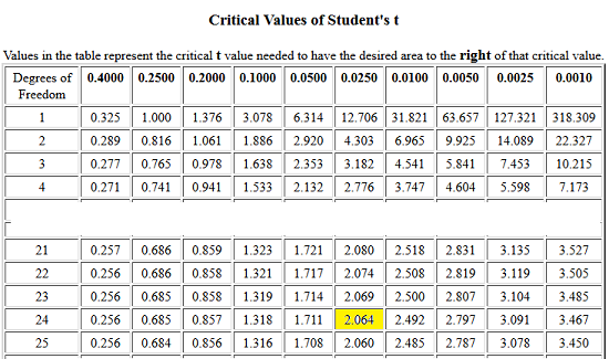
We know that the distribution of sample means, for samples of size 25, will have its mean equal to `mu` and its standard deviation, the standard error, equal to `s_x/sqrt(25)`, and it will be distributed as a Student's t with 25-1 degrees of freedom. Here is an abbreviated table giving t-values for various probabilities and for a select number of degrees of freedom:
At this point we can proceed in either of two ways. First, we can compute the margin of error `t_(alpha/2)xx(s_x/sqrt(n)) = 2.064xx(5.6/sqrt(25))`. That value is the most that our sample mean can differ from the value of `mu` in our null hypothesis. Thus, if we subtract that value from 26 we will have the lowest allowable value for our sample mean; if we add that value to 26 we will have the highest allowable value for our sample mean. Once we know those values we can inspect the sample mean, in this case, 23.5, to see if it is below the lowest allowed value or above the highest allowed value. If either is true then we can reject `H_0: mu=26` in favor of the alternative hypothesis `H1: mu!=26`.
Alternatively, we could just compute the `t`-score of our sample mean, that is, compute `(barx-mu)/(s_x/sqrt(n))=(23.5-26)/(5.6/sqrt(25))` and then compare that value to `-2.064` and to `2.064`. If our computed `t`-score is less than `-2.064` or greater than `2.064`, then we can reject the null hypothesis `H_0:mu=26` in favor of the alternative hypothesis `H_1:mu!=26`.
Let us look at doing these computations on the calculator.

| In Figure 1 we start with computing our margin of error, `2.064xx(5.6/sqrt(25))`, and storing that value into the variable X. Then we find the lower and upper limits on acceptable values for our sample mean. In Figure 1 we see that the lower value is 23.68832 while the upper value is 28.31168. We compare our sample mean, 23.5, to these and we see that the sample mean is actually less than the lower acceptable limit, 23.68832. Thus, from our computations in Figure 1 we reject the null hypothesis in favor of the alternaitve hypothesis. |
 |
Figure 2 demonstrates the other method of analysis. Here we compute our `t`-value as `(23.5-26)/(5.6/sqrt(25))` and we find that value to be `-2.142857143`. We compare this to the the `t`-score from the table, namely, `2.064` and its opposite, namely, `-2.064`. Because our computed `t`-score, `-2.142857143` is less than the lower value, `-2.064`, we reject the null hypothesis in favor of the alternative hypothesis. |
 |
Figure 2a was generated on a TI-84 with the newest software.
This figure shows the DIST menu, with item 4 highlighted.
Press  to select that item. to select that item.
|
 |
The TI-84 responds with this input screen, asking us for the desired area to the left of the `t`-value, and the degrees of freedom. |
 |
In Figure 2c we have supplied the appropriate values. Note that we gave the
calculator the .975 value as the area to the left of the `t`-value,
meaning that we will have 0.025 to the right of that value. The highlight
has been moved down to the
Paste option. Press |
 |
Figure 2d shows the invT( command as the calculator has formed it from the input screen of
Figure 2c. We press to perform the command.
|
 |
The result is shown in Figure 2e. The value of 2.063898542 is the value that was rounded to 2.064
for the table. Thus, if we have a TI-84 with the newer software, we are able to compute the `t`-value rather than having to look it up in a table. |
 |
For Figure 3 we have found the INVT program in the PRGM menu and we have pasted it
onto the main screen. Press
to actually run the program.
|
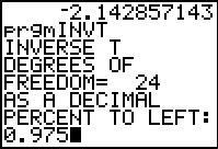 |
The INVT program asks us for the degrees of freedom. We respond with 24. Then the program asks us for the desired area to the left of the `t`-value, and we have responded, in Figure 4 with the value 0.975. |
 |
Not shown between Figure 4 and Figure 5 is the series of dots that the calculator
displays while INVT is working. Once it has come reasonably close to the desired value,
the program, as shown in Figure 5, displays the number of degrees of freedom, the desired area
(labeled as GOAL PERCENT), the `t`-value, in this case 2.063898683, and the area
to the left of that value.
You might notice that the value shown in Figure 5 is slightly different from the value computed by the TI-84 used to produce Figure 2e. This is because the INVT program just tries to get reasonably close to the appropriate value and it gives up before it achieves the accuracy of the internal computations done on the TI-84. Remember that the table value was a much less accurate 2.064. We will not worry about the INVT value being just slightly different from the invT( answer. |
A second program, ASTUDT, was suggested by Jim Egan here at Washtenaw Community College. Rather than do a successive approximation, as does the INVT program, the ASTUDT program uses the available TInterval command to "trick" the calculator into producing the correct result. Let us look at a run of the ASTUDT program.
 |
As usual, we found the ASTUDT program in the PRGM menu and pasted it to the main screen.
Then we press to run the program.
|
 |
ASTUDT starts by telling us that it has an initial setting of 29 degrees of freedom. We press any key to get off of this page and to continue with the program. |
 |
Figure 8 shows the main menu of the program. From here we can
Our problem requires us to have 24, not 29, degrees of freedom. Therefore we select option 1 to take us to Figure 9. |
 |
The program requests a new number of degrees of freedom. We respond with 24
and then press to move to Figure 10.
|
 |
The ASTUDT program merely confirms our input value and then waits for us to hit any key to return to the menu. |
 |
Figure 11 shows that we have returned to the menu and that we have
highlighted the second option.
We can press to move to that option.
|
 |
Now the program asks for the area to the left of the `t`-value. We give that as .975
and then press to continue.
|
 |
The program responds by telling us that the `t`-value 2.063898542 has .975 area to its left.
We might note two things here. First, the actual computation time (which you cannot see on this
web page of course) is much less than the time needed by the INVT
program shown above. Second, the answer from ASTUDT is exacty the same as the answer that the TI-84
produced via its invT( command.
The program waits for us to hit a key to return to the menu. |
|
|
Back at the menu, we will again select option 2. |
 |
This time we will give the desired area as .025. The program returns with the correct answer `-2.063898542`. Again, press any key to return to the menu. |
 |
The actual problem that we are solving was really a two-tailed test with a level of signifcance at 0.05. Thus, we will have 5% of the area between the low and high values. We can use option 4 to compute the `t`-values based on that 95% value. |
 |
The ASTUDT program asks for the area between the values. We respond
with .95, and the program gives us both values.
Not shown on this page is our return to the menu and our selection of item 5 to QUIT the program. |
All of the work thus far has been to use the calculator to evaluate some expressions and to use the calculator to produce the values that we would generally look up in a table. However, there is a feature on the calcualtor that makes all of this seem like extra work. In particular, the calculator has a STAT Tests feature called T-Test.
 |
In Figure 17 we have moved to the STAT menu and then shifted it to the TESTS submenu. There, in position 2, we find the T-Test... option. We select that option to move to Figure 18. |
 |
Figure 18 shows the input form for the T-Test feature. At the moment we have not placed any of our values into this form. We do so to move to Figure 19. |
 |
In Figure 19 we have told the input form that
to perform the command.
|
 |
The result is shown in Figure 20. That Figure gives `H_1:mu_1!=26`,
the `t`-score as `t=-2.23214857`,
the probability of having a `t`-score like that or more extreme
(including having one that is greater than
`2.2314857`, and then it repeats the sample mean, standard deviation, and size.
Our interprestation of this is that we have a `t`-score that has even less than the 0.05% significance level that we started with. Thus, the statistics from our sample have yielded values that are even more rare than the 0.05 significance level that we had set. Therefore, we would reject the null hypothesis in favor of the alternative hypothesis. |
 |
For Figure 21 we have returned to the T-Test input form and here we have only changed
the second from bottom line. Now we are asking the calculator to
use the same values but to do so based on a one-tailed test because now our alternative hypothesis is
`H_1:mu<26`.
After we move to the Calculate field and press the
calcuator takes us to Figure 22.
|
 |
Everything in Figure 22 is the same as it was in Figure 20 except that the proability of having such a `t`-score or a more extreme score has dropped by half. That is because the only more extreme scores are now those that are less than the computed `t`-score. Because the Alternative Hyposthesis is now `H_1:mu<26` we only look at extreme values as being those way less than 26. |
©Roger M. Palay
Saline, MI 48176
November, 2013